PINNs Are Mesh-Free, Not Cost-Free: Stop Replacing Solvers to Feed the GPU Furnace
An opinionated lifecycle-accounting complaint about why PINNs are often oversold as solver replacements, and where scientific machine learning arguments are actually stronger.
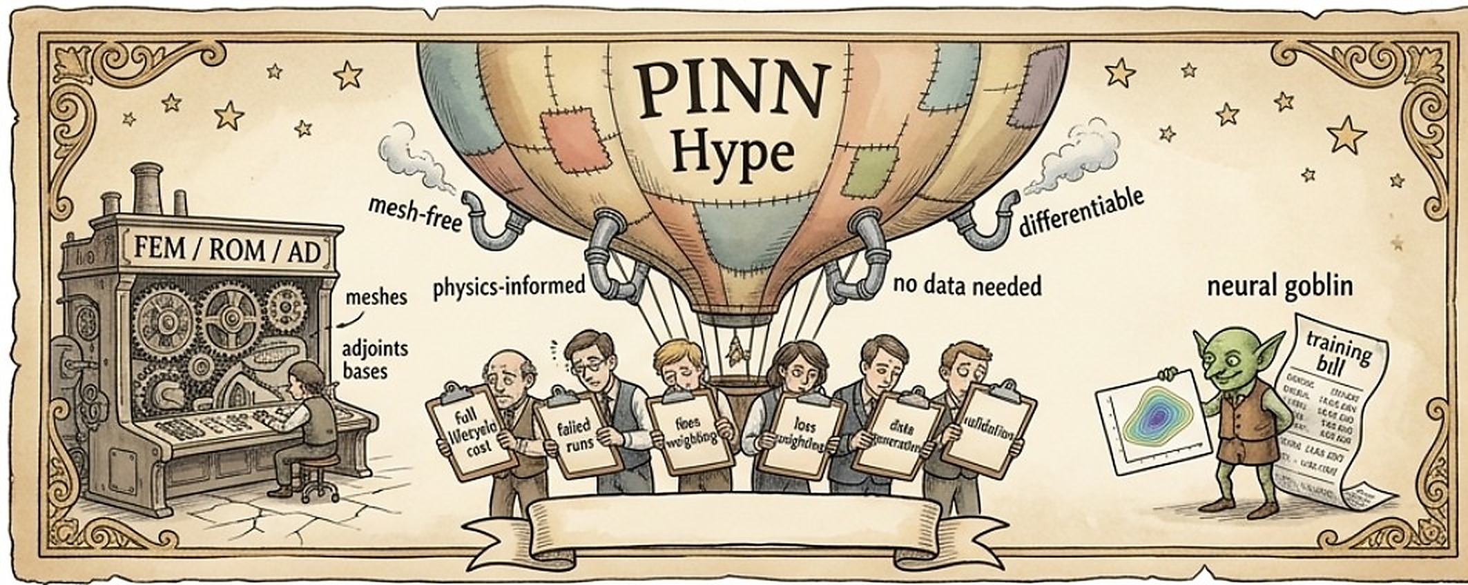
TL;DR
Physics-informed neural networks are often sold as mesh-free, differentiable alternatives to classical solvers. But mesh-free is not cost-free: once training, architecture search, loss balancing, failed runs, data generation, validation, and lifecycle maintenance are counted, PINNs rarely look like a serious replacement for trusted FEM, FVM, FFT, ROM, or adjoint-based workflows. The case for PINNs is not solver replacement. It is narrower, less glamorous, and more useful: physics-regularized regression, inverse prototyping, and hybrid scientific machine-learning workflows where classical solvers remain the source of discipline rather than the thing being theatrically replaced.
Paper-style abstract
Physics-informed neural networks (PINNs) are frequently presented as mesh-free, differentiable, data-efficient alternatives to classical numerical solvers. This framing is attractive, but incomplete. Mesh-free is not cost-free. A fair assessment must include the full lifecycle cost of formulation, architecture selection, optimizer tuning, loss weighting, failed training runs, synthetic data generation, validation, deployment, and maintenance. Under such accounting, PINNs are rarely convincing replacements for mature FEM, FVM, FFT, ROM, or adjoint-based methods in standard forward or inverse engineering workflows. Their differentiability is also not, by itself, evidence of trustworthy sensitivities, especially outside a carefully validated parameter region. This article argues that the useful role of PINNs is narrower than the current hype suggests: physics-regularized regression, sparse-data inverse prototyping, and hybrid scientific machine-learning pipelines. The goal should not be to replace trusted solvers with GPU-hungry residual minimizers, but to use physics-informed models where they add measurable value to accuracy, robustness, uncertainty handling, or workflow efficiency. Otherwise, we are not advancing computational science. We are feeding the GPU furnace with prettier contour plots.
Opening the Balloon
Physics-informed neural networks, or PINNs, are one of those ideas that are very easy to admire from a safe distance. The pitch is clean: take a neural network, feed it spatial and temporal coordinates, use automatic differentiation to evaluate a governing equation, and penalize the residual. Add boundary and initial conditions. Stir with Adam, finish with L-BFGS, and serve as a continuous, differentiable solution field. It is a beautiful recipe. It is also, in too many engineering discussions, a recipe confused with a meal.
The purpose of this article is not to insult researchers working on PINNs. Many of the best PINN papers are careful, mathematically interesting, and honest about limitations. The target here is the surrounding weather system: the inflated claims, incomplete baselines, pretty contour plots, and accounting practices in which training time vanishes politely behind the curtain while inference time arrives wearing a medal. The field deserves better than applause for replacing a certified numerical workflow with a neural interpolant that happens to know how to differentiate itself.
The basic PINN idea is real. Raissi, Perdikaris, and Karniadakis framed PINNs as a deep-learning approach for forward and inverse nonlinear PDE problems, combining data mismatch and physics residual terms in a single loss [1]. That formulation explains why people became excited. It offers one differentiable object into which we can pour sparse measurements, partial physics, unknown coefficients, boundary terms, and hidden states. For inverse problems and data assimilation, that is genuinely attractive. The trouble begins when this convenience is quietly promoted into superiority. A method can be elegant, useful, and overmarketed at the same time. Academia, being a reliable manufacturer of such contradictions, has managed all three.
PINNs Are Often Sold as Solvers. They Are Usually Not Very Good Solvers.
The cleanest case against PINN maximalism is the forward problem. If the governing equations, geometry, material parameters, boundary conditions, and loading are known, the task is simply to solve the PDE. In that regime, finite element, finite volume, spectral, finite difference, boundary element, and FFT-based methods are not historical curiosities. They are the accumulated machinery of several decades of error analysis, preconditioning, adaptivity, conservation, stabilization, meshing, and industrial validation. PINNs enter that arena with a loss function and a dream.
Direct comparisons have not been kind to the dream. Grossmann and co-authors systematically compared PINNs and finite elements on several PDEs, including Poisson, Allen-Cahn, and semilinear Schrodinger examples. Their conclusion was not that PINNs had discovered a secret computational shortcut. In solution time and accuracy, PINNs did not outperform FEM in their study, although trained networks could evaluate a solved field quickly afterward [2]. That is useful for some amortized settings, but it is not the same as beating a solver. Buying a factory to make one sandwich is still a strange lunch strategy.
The optimization pathologies are not accidental blemishes. Krishnapriyan et al. showed that PINNs may handle simple problems and then fail on only moderately harder convection, reaction, and diffusion systems; their evidence points to hard optimization induced by the soft PDE-regularization setup rather than a mere lack of network expressivity [3]. Wang, Yu, and Perdikaris analyzed training through the neural tangent kernel and found that different loss components can converge at very different rates, which helps explain the recurring ritual of loss-weight tuning [4]. In other words, the problem is not only that the network must represent the solution. It must also negotiate a badly conditioned treaty among data, residuals, boundary conditions, and initial conditions. Negotiations go about as well as expected.

The Missing Ledger
The strongest criticism of PINN evidence is not that PINNs never work. It is that many comparisons do not count the full cost of making them work. A fair engineering comparison should include the complete lifecycle: formulation, data generation, architecture selection, collocation strategy, loss weighting, optimizer choice, failed training runs, validation, uncertainty assessment, deployment, maintenance, and the cost of explaining to reviewers why the third random seed retired from public life. Too often the comparison is trained-PINN inference time against one high-fidelity solve. That is not a cost analysis. That is a magic trick with a GPU invoice.
A more honest total cost expression would include data generation from direct numerical solvers or experiments; hyperparameter and architecture exploration; optimizer schedules; domain-decomposition choices; residual sampling; post hoc filtering of failed runs; and validation against trusted numerical or experimental data. Classical inverse methods also have costs, of course: discretization, adjoint or sensitivity implementation, regularization, solver configuration, mesh refinement, and UQ. But these costs are usually explicit. In many PINN papers, the equivalent costs are dissolved into phrases such as 'we trained the model' or 'after tuning'. The small words do astonishing amounts of unpaid labor.
This matters most in inverse problems, where PINNs are often defended more plausibly than in forward solves. There are indeed inverse-flow demonstrations, including hidden-fluid-mechanics style reconstruction and hemodynamic examples where sparse measurements and uncertain boundary conditions make the problem difficult [5,6]. But the relevant question is not whether a PINN can be made to infer something. The question is whether it is better, cheaper, more reliable, and easier to validate than classical inverse methods in the same domain. A recent comparison by Jekic and co-authors tested PINNs against a traditional FEM-plus-optimizer approach on inverse fluid-mechanics problems and found the traditional approach outperformed PINNs, while noting that PINNs may require less human effort and that the gap can shrink in higher-dimensional, data-richer regimes [7]. That is a nuanced result. Naturally, nuance is less popular than a heat map.
Inverse Problems Already Had Adults in the Room
Inverse problems did not begin in 2019 when neural networks discovered partial derivatives. Engineers and applied mathematicians already had adjoints, PDE-constrained optimization, Tikhonov and total-variation regularization, Bayesian inversion, ensemble Kalman methods, 4D-Var, reduced-order data assimilation, parameter estimation, and domain-specific identification tools. These methods are not universally easy, but they come with a culture of identifiability, regularization, sensitivity, uncertainty, and error. That culture is not decorative. It is the difference between knowing what you inferred and merely obtaining a plausible field.
For sparse sensor reconstruction, Gaussian processes and kriging offer strong baselines, especially in low-to-moderate dimensions. They provide uncertainty estimates, explicit covariance assumptions, and kernels that can encode smoothness or physical structure [8]. Polynomial chaos expansions can be excellent when the uncertain parameter dimension is moderate and the solution map is sufficiently smooth, offering spectral-style convergence in favorable cases and clear variance decompositions for uncertainty quantification [9]. Reduced-basis and POD-style methods provide a mature offline-online story for parametric PDEs, often with a posteriori error estimators or certification machinery [10,11]. These methods are not always glamorous, which is unfortunate for them but excellent for engineering.
A PINN can act as a physics-regularized interpolator. That statement is true and sometimes useful. It is also not enough. A shallow neural network with physics-aware features, a constrained Gaussian process, a reduced-order model, splines with weak-form constraints, or a classical data-assimilation method may achieve similar or better performance at lower lifecycle cost. If a PINN paper compares against a naive dense network and declares victory, the victory belongs mostly to baseline selection. This is the scientific equivalent of arm-wrestling a chair.
Differentiability Is Not a Patent Held by PINNs
One of the most persistent arguments for PINNs is differentiability. A trained network is differentiable with respect to its inputs and parameters, so it seems attractive for optimization, control, and inverse design. But differentiability alone is a low bar. A hallucination can be differentiable. The important question is whether the derivative is the derivative of a trustworthy approximation in the region explored by the optimizer.
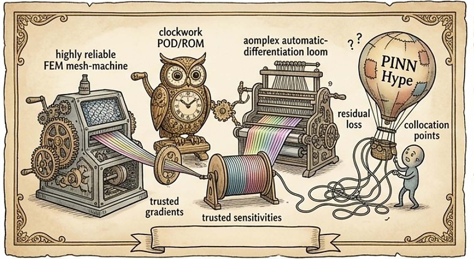
If the goal is differentiable physics, the more compelling path is often to differentiate the solver one already trusts. Enzyme demonstrates automatic differentiation at the LLVM level, generating gradients for statically analyzable programs in languages that lower to LLVM, including C, C++, Fortran, Julia, Rust, Swift, and others [12]. JAX-based differentiable physics and mechanics frameworks show a parallel route: write the numerical model in a differentiable array framework and obtain sensitivities through the simulation workflow [13]. Recent differentiable FEM work in finite-strain anisotropic plasticity reports GPU acceleration and AD-based gradients for inverse characterization, illustrating the obvious but somehow revolutionary idea that the discretization can remain physical while the workflow becomes differentiable [14].
This route changes the comparison. Instead of neural residual fitting versus classical numerics, the question becomes: why not keep the validated discretization, solver structure, constraints, and material integration, then add automatic differentiation, adjoints, or implicit differentiation? A differentiable FEM, FFT-Galerkin, or ROM pipeline can provide gradients of the model engineers actually use. A PINN provides gradients of a neural approximation that may satisfy sampled residuals and still give misleading sensitivities. In design loops, optimizers are talented at finding surrogate lies. They do not need encouragement.
Operator Learning Is the Better Argument, but PINNs Are Not the Only Guest
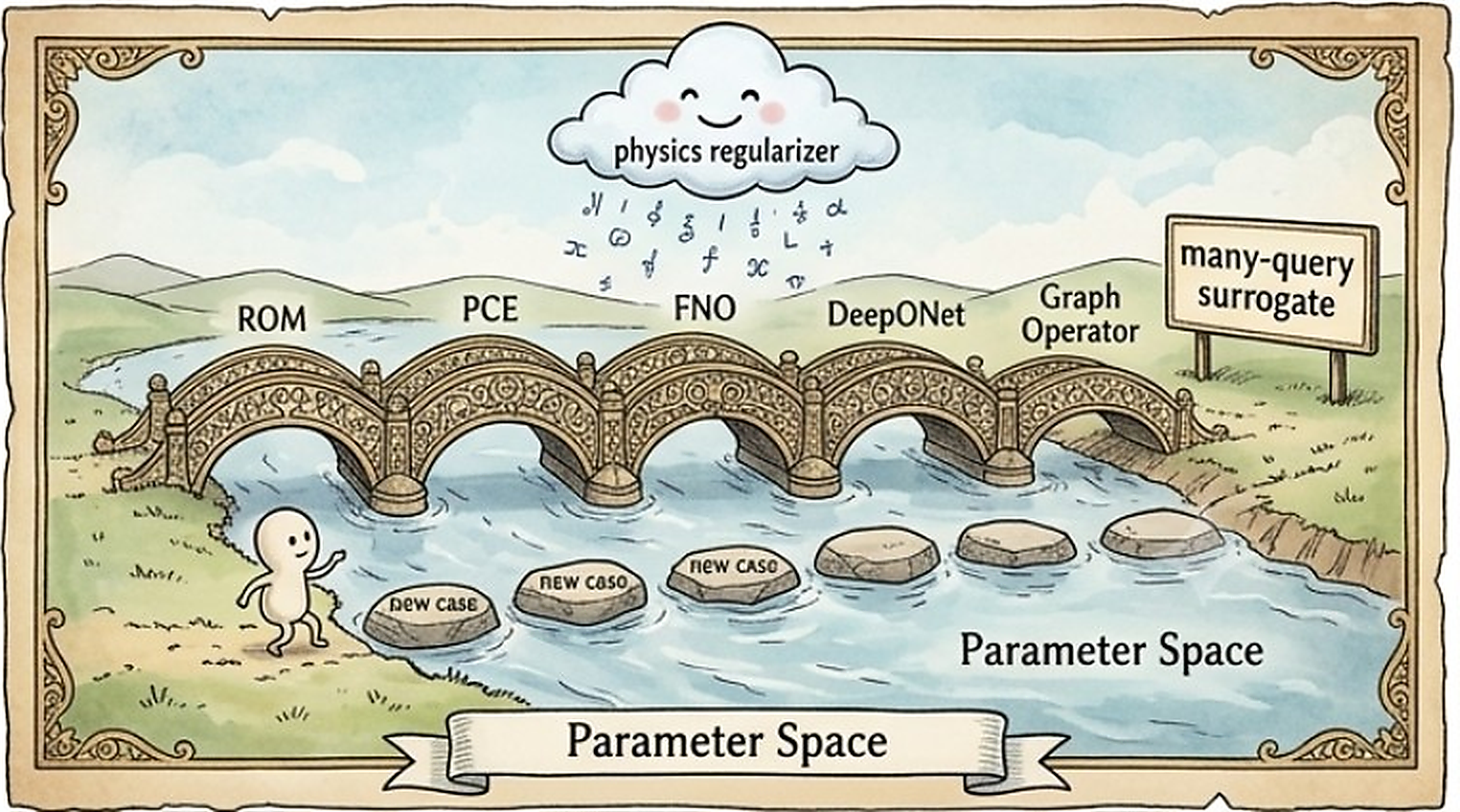
The best place to move the discussion is operator learning. A vanilla PINN often learns one solution field for one problem instance. Change the geometry, loading, parameters, material law, or boundary conditions, and the network may need retraining. That is not generalization in the engineering sense. It is a nonlinear solve wearing a neural costume. Operator learning instead targets the map from inputs such as coefficients, loads, domains, or boundary conditions to output fields. DeepONet, neural operators, and Fourier neural operators were proposed precisely to learn maps between functions or function spaces rather than one coordinate-to-solution field [15-17].
This distinction matters. If the intended use case is many-query simulation over a family of PDEs, materials, microstructures, loads, or boundary conditions, then learning the operator directly is usually more natural than training one PINN per instance. Physics-informed neural operators combine data and PDE constraints in this setting and treat physics as a regularizer on an operator model rather than as the entire training signal for a single field [18]. That is a more credible direction. It still has serious open problems: robustness, dimensionality, distribution shift, uncertainty, rare events, geometry handling, and experimental noise. But at least the tool is pointed at the right target.
Even there, PINN branding should not be allowed to annex the whole territory. Classical reduced-order models, operator inference, reduced basis, PCE, Gaussian-process emulators, graph neural operators, Fourier operators, and domain-specific surrogates all belong in the comparison. The question is not 'Can we add a PDE residual?' The question is 'What is the best end-to-end operator surrogate under a real budget, with honest validation and known failure modes?' That question is less memeable, which is how one knows it is probably worth asking.
The Structure-Preservation Problem
A residual penalty is not the same thing as a structure-preserving discretization. Classical numerical methods often enforce or control conservation, compatibility, stability, monotonicity, boundary conditions, maximum principles, energy dissipation, frame indifference, and variational consistency. PINNs can be designed to respect some of these properties, but the vanilla recipe usually imposes governing equations as soft losses evaluated at collocation points. Between those points, the model may still misbehave. Near shocks, cracks, interfaces, boundary layers, localization zones, or high-frequency fields, the gap between residual-looking and physics-preserving can become expensive.
The field knows this, which is why many serious PINN developments add back pieces of classical numerical wisdom: weak forms, variational losses, hard boundary constraints, conservative formulations, adaptive sampling, domain decomposition, and hybrid finite-element integration. XPINNs and conservative PINNs use domain decomposition to improve scalability and handle complex or multiscale settings [19]. These are legitimate advances. They also reveal the central irony: the more robust PINNs become, the more they resemble a rediscovery of numerical analysis with extra optimizer drama.
This is not a reason to dismiss hybrid methods. It is a reason to stop pretending the original mesh-free slogan was enough. Mesh-free is not cost-free. Soft-constrained is not structure-preserving. Continuous is not accurate. Differentiable is not reliable. The slogans are short because the missing caveats would not fit on the poster.
Where PINNs Still Make Sense
A sober view does leave a useful niche. PINNs can be attractive for fast prototyping of physics-constrained inverse problems when no mature inverse solver is available, when the data are sparse or awkward, when the PDE is only partially known, or when the goal is approximate field reconstruction rather than certified simulation. They may help experimentalists combine scattered observations with physical priors without writing a full adjoint solver. They may be useful inside hybrid workflows where a classical solver validates, corrects, or enriches the neural model. They may help formulate exploratory digital twins that continuously assimilate data and estimate hidden quantities. These are real uses. They are just not a revolution in forward engineering simulation.
A reasonable decision rule is simple. If you need one high-fidelity forward solution, use a high-fidelity solver. If you need many-query parametric simulation, start with ROMs, reduced basis, PCE, operator inference, or neural operators. If you need gradients, differentiate the trusted numerical workflow when possible. If you need inverse reconstruction from sparse measurements and no efficient domain-specific inverse method exists, consider PINNs as one candidate. If your evidence consists mainly of smooth contour plots on squares and cubes, please return the confetti to storage.
This also changes how papers should be read. A PINN result is most interesting when the authors make the competing workflows explicit and explain why they were not used, or why they failed under the same constraints. It is much less interesting when the baseline is an unregularized neural net, a coarse grid chosen without care, or a classical solver denied the adaptivity, adjoint, or reduced-order machinery that practitioners would actually deploy. The comparison should be against the competent adult version of the alternative, not its cardboard cutout.
For real engineering workflows, a PINN should have to beat serious baselines: adjoint FEM, differentiable FEM, reduced-order models, Gaussian processes, PCE, neural operators, coarsened solvers, adaptive mesh refinement, and domain-specific inverse methods. It should report full lifecycle cost, not just inference time. It should disclose failed runs, tuning effort, sensitivity to architecture, optimizer schedules, and loss weights. It should test out-of-distribution behavior and local derivative reliability. It should validate against the solver or experiment that engineers actually trust. These are not hostile requirements. They are the price of being taken seriously.
Conclusion: Deflate Carefully, Then Build Something Better
The case for dropping PINNs is not a case for dropping scientific machine learning. Quite the opposite. It is a case for putting effort where it matters: differentiable solvers, solver-informed surrogates, reduced-order and operator-learning methods, uncertainty quantification, active learning, trustworthy gradients, and hybrid workflows that preserve physical structure. Physics-informed learning should mean more than adding a residual term to a neural network and hoping the optimizer develops professional ethics.
PINNs gave the community a useful abstraction: fit data while respecting equations. That abstraction deserves to survive. The exaggerated claim that PINNs are general replacements for mature solvers does not. Inverse problems, sparse data, and operator learning remain important. But they deserve comparisons against the best available classical and hybrid methods, with all costs counted and all caveats kept in the room. Otherwise we are not doing engineering. We are producing enchanted posters for the conference hallway.
So let us stick a PINN in the hot-air balloon, not because the people building it are foolish, but because the balloon has been asked to carry too much. Keep the useful basket: physics-regularized learning, differentiable programming, data assimilation, and operator surrogates. Let the hot air escape: solver replacement rhetoric, cherry-picked baselines, missing cost ledgers, and contour plots that become persuasive only after enough inconvenient details have been cropped away. The result will be less magical, less marketable, and much more useful. Naturally, this means it will be harder to publish.
References
- Raissi, M., Perdikaris, P. and Karniadakis, G. E. (2019). Physics-informed neural networks: A deep learning framework for solving forward and inverse problems involving nonlinear partial differential equations. Journal of Computational Physics, 378, 686-707.
- Grossmann, T. G., Komorowska, U. J., Latz, J. and Schönlieb, C.-B. (2024). Can physics-informed neural networks beat the finite element method? IMA Journal of Applied Mathematics, 89(1), 143-174.
- Krishnapriyan, A. S., Gholami, A., Zhe, S., Kirby, R. M. and Mahoney, M. W. (2021). Characterizing possible failure modes in physics-informed neural networks. Advances in Neural Information Processing Systems.
- Wang, S., Yu, X. and Perdikaris, P. (2020). When and why PINNs fail to train: A neural tangent kernel perspective. arXiv:2007.14527.
- Raissi, M., Yazdani, A. and Karniadakis, G. E. (2020). Hidden fluid mechanics: Learning velocity and pressure fields from flow visualizations. Science, 367(6481), 1026-1030.
- Arzani, A., Wang, J.-X. and D'Souza, R. M. (2021). Uncovering near-wall blood flow from sparse data with physics-informed neural networks. Physics of Fluids, 33, 071905.
- Jekic, A., Natsaridou, A., Riemer-Sørensen, S., Langseth, H. and Gundersen, O. E. (2025). Examining the robustness of physics-informed neural networks to noise for inverse problems. arXiv:2509.20191.
- Rasmussen, C. E. and Williams, C. K. I. (2006). Gaussian Processes for Machine Learning. MIT Press.
- Xiu, D. and Karniadakis, G. E. (2002). The Wiener-Askey polynomial chaos for stochastic differential equations. SIAM Journal on Scientific Computing, 24(2), 619-644.
- Quarteroni, A., Manzoni, A. and Negri, F. (2016). Reduced Basis Methods for Partial Differential Equations: An Introduction. Springer.
- Kärcher, M., Boyaval, S., Grepl, M. A. and Veroy, K. (2018). Reduced basis approximation and a posteriori error bounds for 4D-Var data assimilation. arXiv:1802.02328.
- Moses, W. S. and Churavy, V. (2020). Instead of rewriting foreign code for machine learning, automatically synthesize fast gradients. arXiv:2010.01709.
- Schoenholz, S. S. and Cubuk, E. D. (2019). JAX MD: A framework for differentiable physics. arXiv:1912.04232.
- Sharma, D., Salgado, I., Huang, L., Wang, H.-P. and Cao, J. (2026). A differentiable GPU-accelerated finite element framework for inverse characterization of finite-strain anisotropic plasticity. arXiv:2606.17390.
- Lu, L., Jin, P. and Karniadakis, G. E. (2019). DeepONet: Learning nonlinear operators for identifying differential equations based on the universal approximation theorem of operators. arXiv:1910.03193.
- Kovachki, N., Li, Z., Liu, B., Azizzadenesheli, K., Bhattacharya, K., Stuart, A. and Anandkumar, A. (2021). Neural operator: Learning maps between function spaces. Journal of Machine Learning Research, 24, 1-97.
- Li, Z., Kovachki, N., Azizzadenesheli, K., Liu, B., Bhattacharya, K., Stuart, A. and Anandkumar, A. (2020). Fourier neural operator for parametric partial differential equations. arXiv:2010.08895.
- Li, Z., Zheng, H., Kovachki, N., Jin, D., Chen, H., Liu, B., Azizzadenesheli, K. and Anandkumar, A. (2021). Physics-informed neural operator for learning partial differential equations. arXiv:2111.03794.
- Shukla, K., Jagtap, A. D. and Karniadakis, G. E. (2021). Parallel physics-informed neural networks via domain decomposition. arXiv:2104.10013.