1. Basic Concepts of Signals¶

When choosing a measurement system, we need to pay attention to several factors which will greatly influence our ability to perform the measurement adequately.

More often than not, the factors we will study (i.e. the inputs to the process) will have to be varied in a continuous or discrete manner, and similarly the process output will be monitored over a range of levels.

The three most basic concepts we will address are:

Waveform - the shape/form of the signal.
Amplitude - the range of the measured or controlled quantity.
Frequency - the way the signal varies in time.

You were asked to measure the temperature of a water container as a function of the voltage passed through a heating system connected to it. How do you approach this task? what is the range of temperatures you need to measure? at what rate do you expect the temperature to change? How will those affect your choice of a measurement system?

Before discussing properties and analysis of signals, let us differentiate between an analog and digital signals.

An analog signal is continuous in time. Similarly, the magnitude of the measured signal is continuous within the measure range.

A digital signal is a discrete representation in time of the change in the physical variable. The values a digital signal can obtain are also discrete and are determined by the level of quantization .

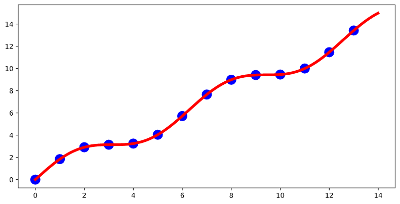
When we sample an analog signal and convert it to a digital signal we represent the signal using a binary representation with a finite number of bits. converting an signal with a range of 5V into a digital signal with \(n\), will result in quantization into \(2^n\) levels.

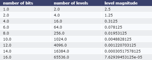
the above table should have been written while keeping in mind the significant digits but it came out pretty so… dont do that its a bad habbit!

Static signals are signals which are (or should be) constant in time. The screen size of your phone for example.

Quasi-static signals are signals whose variation in time is sufficiently slow compared to ….????

Dynamic signals are time dependent. the nature of time dependency of the signal will help us to classify it. Signals can be periodic with just one frequency, or complex periodic suggesting that the signal time dependency is the result of multiple frequencies. Non periodic signals can appear as steps; ramp or pulses. There exist non deterministic signals whose characterization is made following their statistics but we will skip that for now.

1.1. Reminder - properties of periodic signals¶

A periodic function is characterized by:

\(\color{green}{\text{amplitude}}\)
\(\color{blue}{\text{frequency/period}}\)
\(\color{orange}{\text{phase}}\)

Consider a measurment of an AC signal:

\[ y(t) = \color{red}{D} + \color{green}{A} \sin(2 \pi \color{blue}{f} t + \color{orange}{\phi}) =\color{red}{D} + \color{green}{A} \sin( \color{blue}{\omega} t + \color{orange}{\phi}) \]

### import stuff
import numpy as np
import matplotlib.pyplot as plt
from ipywidgets import widgets, interact
from IPython import display
plt.ion()

%matplotlib inline
#### define our function
def PerSig(A, freq,D,phi, samples):
    t=np.linspace(-np.pi, np.pi, samples)
    omega = 2*np.pi*freq
    y=D + A*np.sin(omega*t+phi)
    y1=D + A*np.sin(omega*t)
    fig,ax = plt.subplots(figsize=(10,5))
    ax.plot(t,y,lw=3,label='signal')
    ax.plot(t,y-D,lw=3,label='just the AC component')
    ax.plot(t,y1,lw=3,label='no phase')
    ax.set_xlabel('time')
    ax.set_ylabel('y(t)')
    ax.legend()

interact(PerSig, A = (1,10,1), freq= (0.25, np.pi, 0.2), D=(0,2,1), phi=(0, np.pi, np.pi*0.25), samples=(10,500,10))

<function __main__.PerSig(A, freq, D, phi, samples)>

%matplotlib inline
#### define our function
def ContDis(A, freq,D,phi, samples):
    t=np.linspace(-np.pi, np.pi, 1000)
    t1=np.linspace(-np.pi, np.pi, samples)
    omega = 2*np.pi*freq
    y=D + A*np.sin(omega*t+phi)
    y1=D + A*np.sin(omega*t1+phi)
    fig,ax = plt.subplots(figsize=(10,5))
    ax.plot(t,y,lw=3,label='continous')
    ax.stem(t1,y1,label='discrete')
    ax.plot(t1,y1,lw=3,label='discrete')
    ax.set_xlabel('time')
    ax.set_ylabel('y(t)')
    ax.legend()

interact(ContDis, A = (1,10,1), freq= (0.25), D=(0), phi=(0, np.pi, np.pi*0.25), samples=(3,100,3))

<function __main__.ContDis(A, freq, D, phi, samples)>

1.2. Nyquist Shannon sampling theorem¶

To sample data from a phenomenon whose highest frequency is \(f_{phen}\), the sampling frequency \(f_{samp}\) is :

\[ f_{samp} \geq 2*f_{phen}\]

ME034044notes

1. Basic Concepts of Signals¶

1.1. Reminder - properties of periodic signals¶

1.2. Nyquist Shannon sampling theorem¶